16  Uniform Distribution

16.1 Introduction

So far, we’ve discussed several types of distributions that model different aspects of randomness. The Binomial and Geometric distributions for example, describe the number of successes or failures in repeated experiments, and the Poisson distribution models the number of rare events occurring within a given time frame.

Each of these distributions gives us a way to understand uncertainty, but they all share a common feature: some outcomes are more likely than others. For example, in the Poisson distribution, getting 0, 1, or 2 events might be more likely than getting 10. Similarly, in the Binomial case, getting almost half heads and half tails is more likely than getting all heads.

In this chapter, we explore a different type of distribution, in which every outcome is equally likely. This is called the Uniform distribution. More specifically, we will discuss both the discrete and continuous versions of the Uniform distribution, show examples of how and when they are used, and illustrate how to work with them in R. Despite its simplicity, the Uniform distribution is important in simulations, random sampling, and even in generating more complex distributions.

16.2 When do we encounter the Uniform distribution?

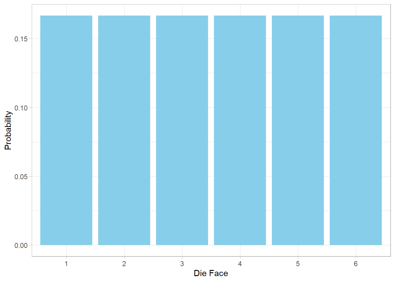
Suppose we are playing a board game and roll a standard six-sided dice. Each of the six possible outcomes, from 1 to 6, has an equal chance of showing up. Since there are six options, each one has a probability of 1/6. This setup is known as a discrete Uniform distribution, because the possible outcomes are distinct and countable.

We can visualize this using a simple bar plot:

In this plot, all bars are of equal height, showing that no face of the dice is more likely than the others. This evenness is the hallmark of the discrete uniform distribution.

Now imagine a different kind of randomness. Let’s say we write a computer program that picks a number completely at random between 0 and 1. We could get 0.2, or 0.9974, or even 0.00005. The important detail is that every number in this interval is equally likely. This is called a continuous Uniform distribution and we can visualize this below:

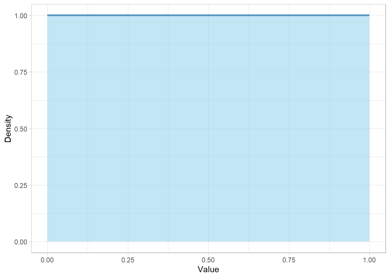
This flat horizontal line represents equal probability across the entire range. No number is more likely than another—just like with the dice before, but now stretched across a continuous space.

16.3 What are the parameters and shape of the Discrete Uniform distribution?

When a variable follows a discrete Uniform distribution, its values can be within a specific range. As such, the minimum and maximum values of that range are the parameters of that distribution. The notation is therefore the following:

\[ X \sim Uniform(a, b) \]

where \(a\) is the minimum value and \(b\) is the maximum value of that range. This means that \(X\) can take on any of the integers in the set \(\{a, a+1, \dots, b\}\), and each value is equally likely. If there are \(n = b - a + 1\) possible values, then the probability mass function of a variable \(X\) is:

\[ P(X = k) = \frac{1}{b-a+1} \]

where \(k = a, a + 1, \dots, b\).

So, for example, if \(X \sim \text{Uniform}(1, 6)\) (a fair dice), then there are \(6\) possible outcomes, each with a probability of \(1/6\).

One of the nice features of the discrete Uniform distribution is that we can directly calculate its mean and variance based on the endpoints \(a\) and \(b\). The formulas of the expected value and the variance are the following:

\[ E(X) = \frac{a + b}{2} \]

\[ Var(X) = \frac{(b - a + 1)^2 - 1}{12} \]

The formula of the expected value is just the midpoint of the range, since the distribution is symmetric. However, the formula of the variance may look more technical, but it captures how the spread increases as the range from \(a\) to \(b\) grows. A wider interval leads to a more spread-out distribution, which is exactly what variance measures.

Why 12?

We may wonder why divide by 12 in the formula for the variance of a discrete uniform distribution. This number isn’t just random. It comes from the math behind how spread-out equally spaced numbers are. When we calculate variance, we’re looking at how much each number differs from the average. In a uniform distribution, the numbers are evenly spaced (like 1, 2, 3, …, 6), so there’s a nice symmetry. Mathematicians figured out long ago that if you take all these evenly spaced numbers, square their distances from the mean, and average them, the pattern always leads to a factor of 12 in the denominator. So, the 12 is part of a neat shortcut that reflects the symmetry and spacing of the numbers. Fortunately, we don’t need to remember where it comes from, but it’s helpful to know that it’s not arbitrary—it shows up naturally from the structure of the uniform distribution.

As an example, suppose \(X \sim Uniform(1, 6)\). The probability of getting a 6 is:

\[ P(X = 6) = \frac{1}{6-1+1} = \frac{1}{6} \]

Additionally, the expected value and variance are the following:

\[ E(X) = \frac{1 + 6}{2} = 3.5 \] \[ Var(X) = \frac{(6 - 1 + 1)^2 + 1}{12} = \frac{35}{12} \approx 2.92 \]

So, while each face (1 through 6) is equally likely, the distribution still has a well-defined average and a measurable amount of variability around it.

16.4 What are the parameters and shape of the Continuous Uniform distribution?

Just like in the discrete case, the continuous Uniform distribution describes outcomes that are equally likely—but this time, over a continuous interval rather than as a set of discrete values. Instead of a dice roll or a count of objects, now we’re talking about measuring something like time, length, or temperature, where the values can fall anywhere within the real-number range.

As with the discrete Uniform distribution, the notation is the following:

\[ X \sim Uniform(a, b) \]

Here, \(a\) and \(b\) are still the minimum and maximum of the interval, but now \(X\) can take any real number in the continuous range \([a, b]\) not just whole numbers.

Because we’re in the continuous world now, we no longer talk about individual probabilities like \(P(X = k)\), since the probability of any single exact value is zero. Instead, we work with the probability density function, which is constant across the interval:

\[ f(x) = \frac{1}{b - a} \]

Here, \(x \in [a, b]\). In this case, the height of the distribution is flat, meaning that every value between \(a\) and \(b\) is equally likely in terms of density.

Just like before, we can compute the expected value and the variance of this distribution:

\[ E(X) = \frac{a + b}{2} \]

\[ Var(X) = \frac{(b - a)^2}{12} \]

We notice that the formula for the expected value is the same as in the discrete case—it’s still the midpoint. The variance formula is slightly different though; instead of \((b - a + 1)^2\), we now use \((b - a)^2\) due to the continuous interval. But just like before, the division by 12 comes from the same mathematical principles—it reflects the spread of a uniform, symmetric distribution.

As an example, suppose \(X \sim Uniform(0, 1)\), which is a special case called the standard Uniform distribution and it’s a foundational tool in statistics and probability. Here’s what we get:

The probability density function is:

\[ f(X) = \frac{1}{1 - 0} = 1 \]

This means the graph is a flat horizontal line at height 1 from 0 to 1. Every value in that interval is equally dense.

The expected value is:

\[ E(X) = \frac{0 + 1}{2} = 0.5 \]

The variance is:

\[ Var(X) = \frac{(1 - 0)^2}{12} = \frac{1}{12} \approx 0.083 \]

Now, what about the probability of getting exactly 0.501?

Since we have a continuous distribution, the probability of hitting any exact number is zero:

\[ P(X = 0.501) = 0 \]

However, the density at that point still exists. Since the probability density function is constant over the interval, the likelihood (density) at \(x = 0.501\) is:

\[ f(0.501) = 1 \]

This tells us that 0.501 is just as “likely” (in terms of density) as any other number between 0 and 1.

16.5 Calculating and Simulating in R

In previous chapters, we introduced how base R uses the prefixes d, r, p, and q to work with distributions. This naming scheme works perfectly for continuous distributions like the continuous Uniform distribution but does not apply directly for discrete Uniform distributions.

Let’s start with a variable \(X\) that follows a standard continuous Uniform distribution over the interval \(x \in [0, 1]\). The probability density function (PDF) for any value in this range is constant at 1:

# Density at 0.001 in Uniform(0,1)
dunif(x = 0.001, min = 0, max = 1)

[1] 1

# Density at 0.501 in Uniform(0,1)
dunif(x = 0.501, min = 0, max = 1)

[1] 1

# Density at 0.999 in Uniform(0,1)
dunif(x = 0.999, min = 0, max = 1)

[1] 1

All of these return 1 because the density is constant for all \(x\) in [0,1].

We can simulate 10 million random draws from this distribution and visualize the density:

# Libraries
library(tidyverse)

# Setting the theme
theme_set(theme_light())

# Setting seed
set.seed(156)

# Simulate 10 million values from Uniform(0,1) distribution
cont_uni_sim <- tibble(x = runif(n = 10000000, min = 0, max = 1))

# Plot the estimated density of simulated values
cont_uni_sim %>% 
  ggplot(aes(x = x)) +
  geom_density() +
  labs(x = "Value",
       y = "Density")

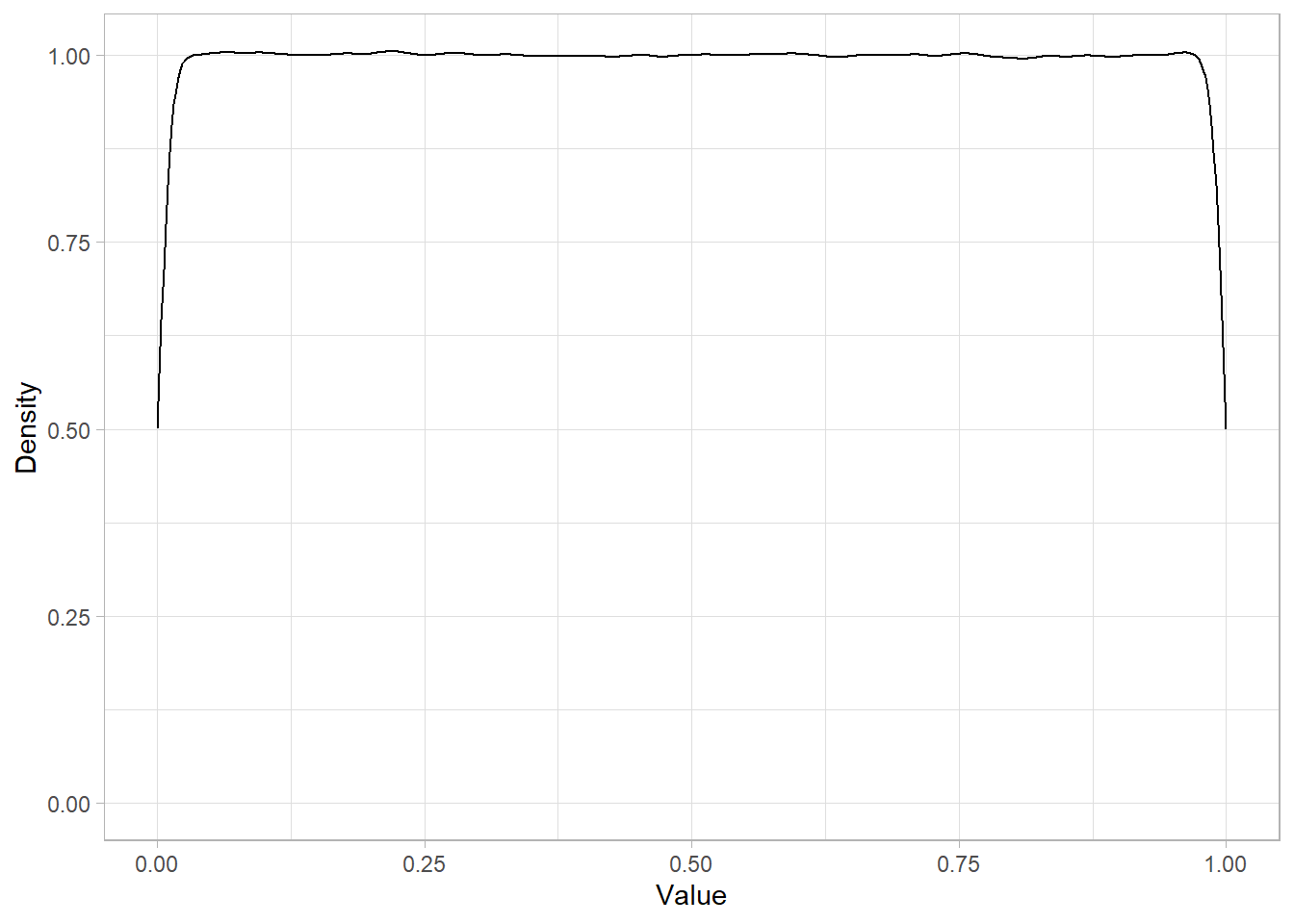
The resulting plot shows a nearly flat density around 1 on the y-axis, reflecting the constant probability density over the interval.

The cumulative distribution function (CDF) gives the probability that \(X\) takes a value less than or equal to some point \(q\):

# Calculate cumulative probability P(X ≤ 0.501) in Uniform(0,1)
punif(q = 0.501, min = 0, max = 1)

[1] 0.501

This returns approximately 0.501, meaning there is about a 50.1% chance that \(X \le 0.501\).

To find the quantile—the value below which a certain percentage of outcomes fall—we use the qunif() function:

# Calculate the 75th percentile (quantile) of Uniform(0,1)
qunif(p = 0.75, min = 0, max = 1)

[1] 0.75

This returns 0.75, indicating that 75% of values fall below or equal to 0.75. This matches perfectly the linear nature of the continuous Uniform distribution.

In R, the simplest way to simulate values from a discrete uniform distribution is the sample() function. This function randomly samples values from a specified vector. Setting replace = TRUE ensures values are drawn independently, as with rolling a die multiple times.

To simulate 10,000 rolls of a fair six-sided die:

# Setting seed
set.seed(123) 

# Simulate 10,000 rolls of a fair 6-sided die
disc_uniform_sim <- sample(x = 1:6, size = 10000, replace = TRUE)

# Plot frequency of each die face
tibble(x = as.factor(disc_uniform_sim)) %>%
  ggplot(aes(x = x)) +
  geom_bar(fill = "skyblue") +
  labs(x = "Die Face",
       y = "Frequency")

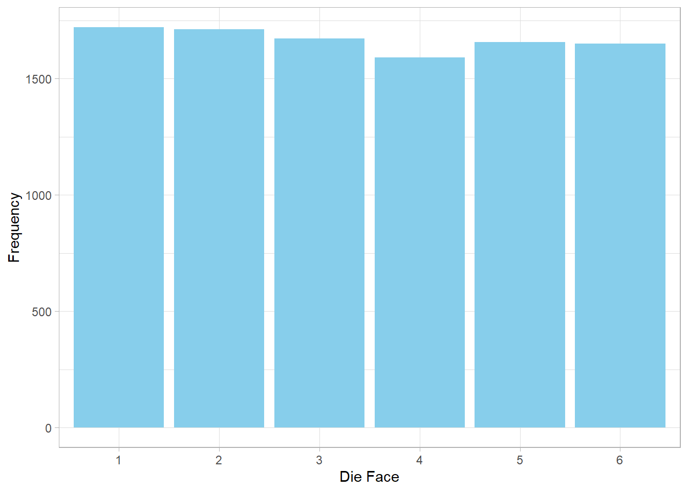
This plot should show roughly equal counts for each face, reflecting the equal probability of each outcome.

Since base R does not have built-in d, p, q functions, we calculate probabilities and cumulative probabilities manually.

The probability of rolling a 5 (the density or PMF) is:

# Create a vector
die <- 1:6

# Probability of rolling exactly 5 on a fair die
mean(die == 5)

[1] 0.1666667

Since all faces are equally likely, each has a probability of \(\frac{1}{6} \approx 0.167\).

To find the cumulative probability of rolling up to 3 (i.e., \(P(X \le 3)\)):

# Cumulative probability up to 3
mean(die <= 3)

[1] 0.5

This means there is a 50% chance of rolling 1, 2, or 3.

Finally, to find the 75th percentile of the discrete uniform over \(\{1, \dots, 6\}\)—the smallest number \(q\) such that at least 75% of outcomes are \(\le q\)—we calculate:

# Find the smallest number q such that P(X ≤ q) ≥ 0.75
# Try each value of die and check which satisfies the condition
percentiles <- sapply(die, function(x) mean(die <= x))

# Get the first die face where cumulative probability ≥ 0.75
die[min(which(percentiles >= 0.75))]

[1] 5

The result is 5, meaning 75% of the rolls will land at 5 or below.

16.6 Recap

In this chapter, we discussed the Uniform distribution, a fundamental probability distribution where all outcomes are equally likely. We explored both the discrete version—used when outcomes are countable, like rolling a die—and the continuous version, where values can take on any number within a given interval, like a random decimal between 0 and 1.

We saw that in both cases, the probability (or density) is spread evenly across the range of possible values. We also introduced formulas for calculating the expected value and variance, showing how these depend on the endpoints of the distribution. The symmetry of the Uniform distribution makes its properties especially intuitive.

Finally, we demonstrated how to simulate and analyze Uniform distributions using R, including visualizations, random number generation, and cumulative probabilities. This simple but powerful distribution is a key building block in probability, simulation, and many real-world applications.